Human Induced Climate Change Experiment

The World Bank and UN Security Council on Global Warming Threat

I had the honor of speaking to the UN Security Council about an increasingly dangerous threat facing cities and countries around the world, a threat that, more and more, is influencing everything that they and we do: climate change.

World Bank President Jim Kim is in Russia right now talking with G20 finance ministers about the same thing – the need to combat climate change. Every day, we’re hearing growing concerns from leaders around the world about climate change and its impact.

If we needed any reminder of the immediacy and the urgency of the situation, Australia Foreign Minister Bob Carr and our good friend President Tong of Kiribati spoke by video of the security implication of climate effects on the Pacific region. Perhaps most moving of all, Minister Tony deBrum from the Marshall Islands recounted how, 35 years ago, he had come to New York as part of a Marshall Islands delegation requesting the Security Council’s support for their independence. Now, when not independence but survival is at stake, he is told that this is not the Security Council’s function. He pointed to their ambassador to the UN and noted that her island, part of the Marshall Islands, no longer exists. The room was silent.

It fell to us to point out the security implications of business as usual. If the world does nothing to stop climate change:

  • half the global population will be living in water-scarce countries by the end of the century, compared to 28% today;
  • 35% of sub-Saharan Africa’s cropland will become unsuitable for cultivation, with grave consequences for food security;
  • the breadbaskets of North America and the Mediterranean will see repeats of this past summer’s crop-crumbling heat waves more frequently, to potentially devastating effect.


So what do we do?

First, cities. Developing countries are urbanizing fast – some will be shifting from less than 20% urban today to more than 60% in the next 30 years. The decisions they make today – about transportation infrastructure, water supply, land use rules, building codes and more – will lock in development patterns for decades to come.

They can choose to grow green with careful, integrated urban planning and support – they will need direct finance and assistance. We will need to step up our work here in support of our clients. In China, cities are seizing on low-carbon development options. We’re helping Lagos develop more sustainable transportation.

We will need to change the way we produce our food, as well. The world’s farmers will need to produce 70% more food by 2050 to feed a population expected to pass 9 billion people, and yet climate scientists tell us that for every 1 degree Celsius increase in average temperature around the world, crop yields will decrease by an average of 5%. We can and must farm in ways that increase productivity, build farmers’ ability to cope with erratic weather, and increase carbon storage on land. We are mobilizing global alliances on climate-smart agriculture, and we have no time to lose.

World Bank Vice President for Sustainable Development Rachel Kyte and UN Secretary-General Ban Ki-moon at the Security Council meeting February 15, 2013. Yuvan Beejadhur/World BankWe are also helping countries transition to a cleaner energy mix. We have doubled our investments in renewable energy in the last five years, and the $7.6 billion Climate Investment Funds we administer will support low-carbon, climate-resilient projects in 48 countries. But that $7.6 billion is a drop in the ocean of what is needed to support the transition to green infrastructure and energy systems. The resilient and green infrastructure gap is, after all, calculated at around $1.3 trillion a year – excluding operation and maintenance.

Stopping a 4°C warmer world from becoming reality and staying at a 2°C one still requires huge investments in adaptation – effectively the resilience of countries, cities, communities, especially the poor.

Disaster risk management – putting effort into prevention and preparedness rather than simply reacting after disasters strike – saves lives and property, and it is increasingly at the core of the Bank’s work. Preserving wetlands and mangroves provides protective storm barriers. Avoiding development in vulnerable areas prevents flooding and deaths that often affect a community’s poorest residents. Through the Global Facility for Disaster Reduction and Recovery, the Bank is working with client countries to mainstream disaster risk management into their development planning.

We recognize that there is much more we can do. President Kim has challenged us to take bold action. We need to get prices right, get finance flowing, and work where it matters most. Our mission, to end poverty and build shared prosperity, will be futile if we don’t.
Rachel Kyte
Vice President for Sustainable Development
www.worldbank.org/sustainabledevelopment

Posted in Uncategorized | Tagged , , , , , , , , , , , , , , , | Comments closed

Arctic Sea Ice Volume Losses

By George Hale,
NASA Goddard Space Flight Center

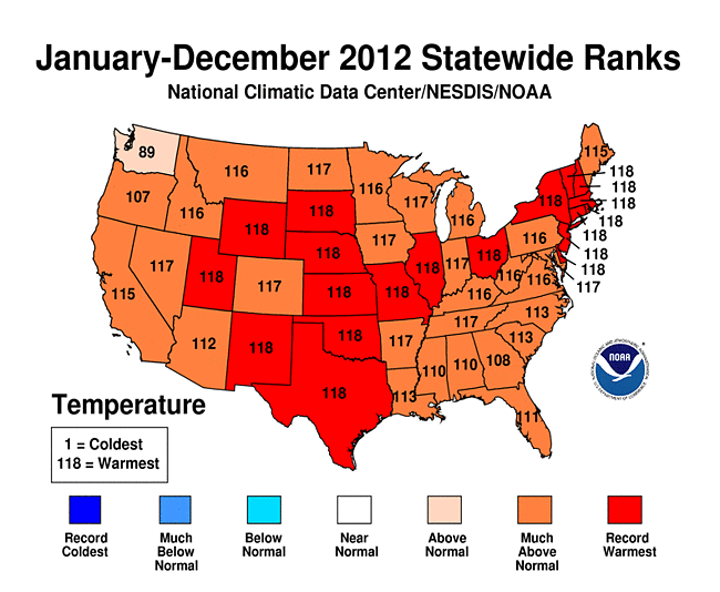
New research using combined records of ice measurements from NASA’s Ice, Cloud and Land Elevation Satellite (ICESat), the European Space Agency’s CryoSat-2 satellite, airborne surveys and ocean-based sensors shows Arctic sea ice volume declined 36 percent in the autumn and nine percent in the winter over the last decade.

The work builds on previous studies using submarine and NASA satellite data, confirms computer model estimates that showed ice volume decreases over the last decade, and builds a foundation for a multi-decadal record of sea ice volume changes.

In a report published online recently in the journal Geophysical Research Letters, a large international collaboration of scientists outlined their work to calculate Arctic sea ice volume. The satellite measurements were verified using data from NASA’s Operation IceBridge, ocean-based sensors and a European airborne science expedition. This was compared with the earlier sea ice volume data record from NASA’s ICESat, which reached the end of its lifespan in 2009.

The researchers found that from 2003 to 2008, autumn volumes of ice averaged 2,855 cubic miles (11,900 cubic kilometers). But from 2010 to 2012, the average volume dropped to 1,823 cubic miles (7,600 cubic kilometers) — a decline of 1,032 cubic miles (4,300 cubic kilometers). The average ice volume in the winter from 2003 to 2008 was 3,911 cubic miles (16,300 cubic kilometers), dropping to 3,551 cubic miles (14,800 cubic kilometers) between 2010 and 2012 — a difference of 360 cubic miles (1,500 cubic kilometers).

The study, funded by the United Kingdom’s National Environmental Research Council, the European Space Agency, the German Aerospace Center, Alberta Ingenuity, NASA, the Office of Naval Research and the National Science Foundation and led by Professor Seymour Laxon of University College London, marks the first ice volume estimates from CryoSat 2, which was launched in 2010. “It’s an important achievement and milestone for CryoSat-2,” said co-author Ron Kwok at NASA’s Jet Propulsion Laboratory in Pasadena, Calif.

Combining the ingredients

Although CryoSat-2 data show a decrease in ice volume from 2010 to 2012, two years is not a long enough time span to determine a trend. This is where NASA’s data and scientists come in. Data from ICESat and IceBridge are freely available, but combining measurements from different sources can be challenging. Kwok said researchers spent months working out how to compare the datasets and making sure they were compatible enough to compare trends. “We participated as collaborators to help interpret results from the datasets we’re familiar with,” said scientist Sinead Farrell at NASA’s Goddard Space Flight Center in Greenbelt, Md.

CryoSat-2 and ICESat both measure sea ice freeboard, which is the amount of ice floating above the ocean’s surface. Researchers use freeboard to calculate ice thickness. This thickness measurement is then combined with ice area to come up with a figure for volume. The two satellites used different methods for measuring freeboard, however. ICESat used a laser altimeter, which bounces a laser off the snow covering the sea ice, while CryoSat-2 uses a radar instrument that measures surface elevation closer to the ice surface. These instruments have a different view of the surface, but researchers found they gave comparable measurements.

Check and double check

Comparing the two datasets and ensuring their quality called for additional data. The two satellites do not cover overlapping time spans, so researchers used measurements from upward-looking sonar (ULS) moorings under the ocean’s surface, located north of Alaska. These instruments, operated by the Woods Hole Oceanographic Institution’s Beaufort Gyre Exploration Project, provide a continuous record of ice draft — thickness of ice below the ocean’s surface — in parts of the Beaufort Sea from 2003 to the present day. Thickness measurements from these ULS moorings were comparable to ICESat and CryoSat-2 data throughout both missions’ time spans. “ULS ice draft since 2003 served as the common data set for cross comparison of the ICESat and CryoSat-2 measurements,” said Kwok.

Researchers took extra care to verify CryoSat-2′s data, as it is a new satellite with a new instrument. In addition to the ULS data, CryoSat-2 measurements were also verified by two airborne science campaigns: flights by an aircraft operated by the Alfred Wegener Institute for Polar and Marine Research in Bremerhaven, Germany; and Operation IceBridge, a NASA mission tasked with monitoring changes in polar ice to bridge the gap in measurements between ICESat and its replacement, ICESat-2, scheduled to launch in 2016. During the 2011 and 2012 Arctic campaigns, the IceBridge team coordinated closely with ESA’s CryoVEx program to verify CryoSat-2 data. “IceBridge was used as a validation tool to understand thickness measurements from CryoSat-2,” said scientist Nathan Kurtz at NASA Goddard Space Flight Center, Greenbelt, Md.

The road ahead

After months of work, researchers had assembled a multi-year dataset, which they could compare to sea ice volume predictions from the Pan-Arctic Ice-Ocean Modeling and Assimilation System (PIOMAS). Because of the short time span of previous satellite studies, researchers have used models like PIOMAS to simulate changes in sea ice volume. The study’s observations show a larger autumn ice volume decrease than predicted, while changes in the winter are smaller than in the model simulation. “It’s important to know because changes in volume indicate changes in heat exchange between the ice, ocean and atmosphere,” said Kurtz.

This study, and the knowledge that the datasets are compatible, also serves to lay groundwork for ICESat-2. CryoSat-2 gathers data over more of the Arctic than ICESat did by reaching 88 degrees north (ICESat reached 86 degrees). ICESat-2 will orbit Earth at the same angle as CryoSat-2 and will therefore survey the same amount of the Arctic.

CryoSat-2 is funded through 2017 but will likely operate until the end of the decade, giving overlapping coverage with ICESat-2. This potential overlap greatly improves the prospects for better knowledge of Arctic sea ice volume. “The hope is that we’ll be able to create a multi-decadal record using ICESat, CryoSat-2 and ICESat-2,” said Kwok.

For more about ICESat, visit: http://icesat.gsfc.nasa.gov/. For more about Operation IceBridge, visit: http://www.nasa.gov/mission_pages/icebridge/index.html. For more about CryoSat-2, visit: http://www.esa.int/Our_Activities/Observing_the_Earth/CryoSat. For more about the Beaufort Gyre Exploration Project, visit: http://www.whoi.edu/page.do?pid=66296.

Posted in Uncategorized | Tagged , , , , , , , , , , , , , | Comments closed

1/5 Of Reptile Species Endangered

Nineteen percent of the world’s reptiles are estimated to be threatened with extinction, states a paper published today by the Zoological Society of London (ZSL) in conjunction with experts from the IUCN Species Survival Commission (SSC).

The study, printed in the journal of Biological Conservation, is the first of its kind summarising the global conservation status of reptiles. More than 200 world renowned experts assessed the extinction risk of 1,500 randomly selected reptiles from across the globe.Out of the estimated 19% of reptiles threatened with extinction, 12% classified as Critically Endangered, 41% Endangered and 47% Vulnerable.

Chamaeleo Hoehneliimichele
©Michele Menegon

Three Critically Endangered species were also highlighted as possibly extinct. One of these, a jungle runner lizard Ameiva vittata, has only ever been recorded in one part of Bolivia. Levels of threat remain particularly high in tropical regions, mainly as a result of habitat conversion for agriculture and logging. With the lizard’s habitat virtually destroyed, two recent searches for the species have been unsuccessful.

Atheris Ceratophoramichele
©Michele Menegon

Dr. Monika Böhm, lead author on the paper: “Reptiles are often associated with extreme habitats and tough environmental conditions, so it is easy to assume that they will be fine in our changing world.

“However, many species are very highly specialised in terms of habitat use and the climatic conditions they require for day to day functioning. This makes them particularly sensitive to environmental changes,” Dr. Böhm added.

Ahaetulla Nasutaruchira
©Ruchira Somaweera

Extinction risk is not evenly spread throughout this highly diverse group: freshwater turtles are at particularly high risk, mirroring greater levels of threat in freshwater biodiversity around the world. Overall, this study estimated 30% of freshwater reptiles to be close to extinction, which rises to 50% when considering freshwater turtles alone, as they are also affected by national and international trade.

Although threat remains lower in terrestrial reptiles, the often restricted ranges, specific biological and environmental requirements, and low mobility make them particularly susceptible to human pressures. In Haiti, six of the nine species of Anolis lizard included in this study have an elevated risk of extinction, due to extensive deforestation affecting the country.

Collectively referred to as ‘reptiles’, snakes, lizards, amphisbaenians (also known as worm lizards), crocodiles, and tuataras have had a long and complex evolutionary history, having first appeared on the planet around 300 million years ago. They play a number of vital roles in the proper functioning of the world’s ecosystems, as predator as well as prey.

Head of ZSL’s Indicators and Assessment Unit, Dr Ben Collen says: “Gaps in knowledge and shortcomings in effective conservation actions need to be addressed to ensure that reptiles continue to thrive around the world. These findings provide a shortcut to allow important conservation decisions to be made as soon as possible and firmly place reptiles on the conservation map,”

“This is a very important step towards assessing the conservation status of reptiles globally,” says Philip Bowles, Coordinator of the Snake and Lizard Red List Authority of the IUCN Species Survival Commission. ”The findings sound alarm bells about the state of these species and the growing threats that they face globally. Tackling the identified threats, which include habitat loss and harvesting, are key conservation priorities in order to reverse the declines in these reptiles.”

The current study provides an indicator to assess conservation success, tracking trends in extinction risk over time and humanity’s performance with regard to global biodiversity targets.

ZSL and IUCN will continue to work with collaborating organisations to ensure reptiles are considered in conservation planning alongside more charismatic mammal species.

Read the paper: The Conservation Status of the World’s Reptiles

Lyriocephalus Scutatusruchira
©Ruchira Somaweera

Posted in Uncategorized | Tagged , , , , , , | Comments closed

One of the Most Extreme Years on Record


2012 National Events Map
Click for more information
 

Issued January 8, 2013: The data presented in this report are final through July and preliminary from August-December. Ranks, anomalies, and percent areas may change as more complete data are received and processed.


National Temperature and Precipitation Analysis


Supplemental 2012 Temperature and Precipitation Information

In 2012, the contiguous United States (CONUS) average annual temperature of 55.3°F was 3.2°F above the 20th century average, and was the warmest year in the 1895-2012 period of record for the nation. The 2012 annual temperature was 1.0°F warmer than the previous record warm year of 1998. Since 1895, the CONUS has observed a long-term temperature increase of about 0.13°F per decade. Precipitation averaged across the CONUS in 2012 was 26.57 inches, which is 2.57 inches below the 20th century average. Precipitation totals in 2012 ranked as the 15th driest year on record. Over the 118-year period of record, precipitation across the CONUS has increased at a rate of about 0.16 inch per decade.

On a statewide and seasonal level, 2012 was a year of both temperature and precipitation extremes for the United States. Each state in the CONUS had annual temperatures which were above average. Nineteen states, stretching from Utah to Massachusetts, had annual temperatures which were record warm. An additional 26 states had one of their 10 warmest years. Only Georgia (11th warmest year), Oregon (12th warmest), and Washington (30th warmest) had annual temperatures that were not among the ten warmest in their respective period of records. A list of the annual temperatures for each of the lower-48 states is available here. Numerous cities and towns were also record warm during 2012 and a select list of those locations is available here. Each state in the CONUS, except Washington, had at least one location experience its warmest year on record. One notable warmest year record occurred in Central Park, in New York City, which has a period of record dating back 136 years.

Much of the CONUS was drier than average for the year. Below-average precipitation totals stretched from the Intermountain West, through the Great Plains, into the Midwest and Southeast. Nebraska and Wyoming were both record dry in 2012. Nebraska’s annual precipitation total of 13.04 inches was 9.78 inches below average, and Wyoming’s annual precipitation total of 8.08 inches was 5.09 inches below average. New Mexico, Colorado, Kansas, Missouri, Illinois, Arkansas, Georgia, and Delaware had a top ten dry year. The large area of dry conditions in 2012 resulted in a very large footprint of drought conditions, which peaked in July with about 61 percent of the CONUS in moderate-to-exceptional drought, according to the Palmer Drought Severity Index (PDSI). The footprint of drought during 2012 roughly equaled the drought of the 1950s which peaked at approximately 60 percent. Wetter-than-average conditions were present for the Northwest, where Washington had its fifth wettest year on record. Washington’s statewide precipitation total of 47.24 inches was 10.40 inches above average. Wetter-than-average conditions were also present across parts of the Gulf Coast and Northeast.

Seasonal highlights in 2012 include the fourth warmest winter (December 2011-February 2012), with warmer-than-average conditions across a large portion of the country. The largest temperature departures from average were across the Northern Plains, Midwest, Mid-Atlantic, and Northeast. Winter was drier than average for the East and West coasts, while the Southern Plains were wetter than average improving drought conditions across New Mexico, Oklahoma, and Texas. The warmer and drier than average conditions resulted in the third smallest winter snow cover extent on record for the contiguous United States. Spring (March-May) was record warm for the country, with 34 states being record warm for the period. The season consisted of the warmest March, fourth warmest April, and second warmest May on record. Spring precipitation was near-average for the lower-48, with the Pacific Northwest and Upper Midwest being wetter than average, while the Central Rockies and Ohio Valley were drier than average. The summer (June-August) continued the warmer-than-average trend for the contiguous U.S. with national temperatures ranking as the second warmest on record. The summer average temperature for 2012 was very close to the warmest summer (2011) and the third warmest summer (1936), with only 0.1°F separating the three. The summer season consisted of the eighth warmest June, record warmest July, and 13th warmest August. Drier-than-average conditions were anchored in the central U.S. with record breaking wildfires and a drought footprint comparable to the drought episodes of the 1950s causing large-scale agriculture problems in the Midwest, Plains, and Mountain West. Autumn (September-November) temperatures were closer to average compared to the preceding three seasons, but still ranked as the 22nd warmest autumn on record. Warmer-than-average conditions were present for the West, while cooler-than-average conditions were present for the Eastern Seaboard. Precipitation totals for the nation averaged as the 22nd driest autumn on record.

This annual report places the temperature and precipitation averages into historical perspective, while summarizing the notable events that occurred in 2012. More detailed analysis on individual months can be found through the Climate Monitoring home page.


Top Ten U.S. Weather/Climate Events for 2012

The following is a list for the top ten U.S. weather/climate events which occurred during 2012. These events were selected by a panel of weather/climate experts from around the country. For additional information on these events, please see our Top Ten U.S. Events webpage.


Rank Event
1 Hurricane/Post-Tropical Storm Sandy
2 Contiguous U.S. Drought
3 Contiguous U.S. Warmest Year on Record
4 Record Wildfire Activity
5 Multi-State Derecho
6 March 2nd-3rd Severe Weather Outbreak
7 Alaska Cold Winter/Snow Records
8 Near-Record Low Great Lakes Levels
9 Contiguous U.S. Snow Cover
10 Hurricane Isaac

Seasonal Analysis


Winter

The 2011/12 winter season was marked by above-average temperatures for a large portion of the nation, stretching from the Rockies, through the Plains, and along the East Coast. The Northern Plains, Midwest, and Northeast had the largest temperature departures from average for the season. The CONUS had an average winter temperature of 36.4°F, which was 3.8°F above the 20th century average and was the fourth warmest winter on record. In total, 22 states had December-February temperatures ranking among their ten warmest and four states in the West had winter temperatures which were near-normal. This winter season contrasted with the previous two winters for the CONUS (2009/10 and 2010/11) which ranked as the 14th and 34th coldest winter seasons, respectively. The 2009/10 and 2010/11 winters were marked by record and near-record negative phases of the North Atlantic (NAO) and Arctic (AO) oscillations, which were associated with frequent and long-lasting cold-air outbreaks. The 2011/12 winter had the opposite configuration of the NAO and AO. The NAO averaged for December 2011 was +2.52, the largest positive phase of the index for a month on record. When the NAO and AO are in a positive phase during the winter, the jet stream, which divides cold Arctic air to the north and warm sub-tropical air to the south, tends to remain north of the U.S.-Canadian border. This was the case for the 2011/12 winter which was marked by few and short-lived cold air outbreaks in the CONUS.

The presence of La Niña during the winter had a minimal influence on precipitation patterns during the season. The 3-month average CONUS precipitation of 5.77 inches was 0.70 inch below average. The western U.S. was drier than average, where California had its third driest winter on record, with a statewide precipitation total of 4.09 inches, 7.82 inches below average. Drier-than-average conditions stretched across the Northern Plains into the Upper Midwest. Much of the Eastern Seaboard was also drier than average, where North Carolina had its ninth driest winter and South Carolina its sixth driest. The warm and dry conditions during winter limited snow across a large portion of the country, and the CONUS had its third smallest seasonal snow cover since satellite records began 46 years ago. Many of the major cities in the Northeast and Midwest had record and near-record low seasonal snowfall. Wetter-than-average conditions occurred in the Southern Plains, where Texas had its tenth wettest winter with a precipitation total of 7.63 inches, 2.50 inches above average. The above-average winter precipitation in Texas helped to improve drought conditions which plagued the state during much of 2011. Above-average precipitation was also present for parts of Ohio Valley. The drier-than-average conditions observed along the East Coast and wetter-than-average conditions in the Ohio Valley are consistent with La Niña, but the winter wetness in the Southern Plains is more typical of an El Niño, not a La Niña.

Spring

The spring (March-May) of 2012 was marked by record warmth over a large portion of the country. The CONUS average temperature for the season was 56.1°F, 5.2°F above the 20th century average, and the warmest spring on record, by 2.0°F. The previous record warm spring occurred in 1910 with a seasonally averaged temperature of 54.1°F. Spring 2012 also marked the largest warm temperature departure from average for any season on record for the CONUS. All three months of the season ranked among their five warmest, also a first for the nation. The March average temperature was 8.6°F above average and the record warmest March, April was 3.6°F above average and the fourth warmest April, and May was 3.5°F above average, the second warmest May on record. Thirty-four states0 were record warm for spring, all east of the Rockies, while an additional eight states were top ten warm. The U.S. Climate Extremes Index (USCEI) was record large for the season, driven mostly by the large footprint in extremely warm daytime and warm nighttime temperatures. Numerous states, mostly across the Midwest, had spring temperatures more than 7.0°F above average. Only Oregon and Washington had seasonal temperatures near normal.

The spring CONUS precipitation total of 7.32 inches was 0.39 inch below average and ranked near the median value. The near-average CONUS precipitation total masked regional extremes on both the wet and dry ends of the spectrum. The Pacific Northwest was bombarded by numerous storms during the spring season, resulting in Oregon and Washington having seasonal precipitation totals among their ten wettest. The active storm pattern resulted in above-average snowpack for the Cascades of Oregon and Washington, with near-normal snowpack stretching eastward through the northern Rockies of Idaho, Montana, and northern Wyoming. The Upper Midwest was also wetter than average, where Minnesota had its third wettest spring. Below-average precipitation totals were centered in the central Rockies and the Ohio Valley. Colorado, Utah, and Wyoming each had a top ten dry spring season, where below-average snowpack resulted. In the Ohio Valley, Indiana and Tennessee both had a top ten dry spring. The below-average precipitation in the Midwest was accompanied by below-average tornado activity, despite a few deadly tornado outbreaks. The warm and dry spring, in combination with other factors, played precursor to the large expansion of drought which impacted the nation during the summer of 2012.

Summer

The summer (June-August) of 2012 brought a continuation of warmer-than-average conditions for a large area of the CONUS. The summer’s average temperature for the CONUS was 73.8°F, 2.6°F above the 20th century average and the second warmest summer on record. Only the summer of 2011 was warmer. Above-average temperatures were present for the Rockies, Great Plains, Midwest, Northeast, and much of the West, with the exception of Washington State. The Southeast had near-normal summer temperatures. Colorado and Wyoming each had their warmest summer on record, with 3-month average temperatures 4.9°F and 4.6°F above average, respectively. Twenty-one additional states had summer temperatures among their ten warmest. During the summer, at least 357 all-time hot daytime temperature records were broken, including a new all-time state record for South Carolina (113.0°F). During the summer period, approximately 99.1 million Americans experienced at least 10 days with daytime temperatures exceeding 100.0°F — nearly one third of the country’s population. In addition to the warm summer, the period from August 2011 through July 2012 was the warmest consecutive 12 months that the nation has observed.

In addition to the summer being hot for a large part of the country, it was also dry, resulting in a drought footprint comparable to the drought episodes of the 1950s. The drought peaked in July, when according to the Palmer Drought Severity Index (PDSI), the spatial area of the CONUS in at least moderate drought was 61.8 percent. The summer CONUS precipitation total of 7.22 inches was 1.03 inches below average and the 14th driest summer on record. The epicenter of the drought stretched from the Rockies through the Great Plains and into the Midwest. Wyoming and Nebraska had their driest summer on record with precipitation totals 44 percent and 39 percent of average, respectively. Six additional states had summer precipitation totals among their ten driest. The hot and dry conditions also caused significant wildfire activity across the nation. The 7.0 million acres which burned during the three summer months was the second most in the 13-year record, slightly behind the summer of 2005. The West Coast was slightly wetter than average during the summer, where an active storm pattern in the Northwest, and an active monsoonal flow in the Southwest kept conditions wet. The Gulf Coast was wetter than average, with Florida having its wettest summer on record with a seasonal precipitation total 140 percent of average. The summer wetness along the Gulf Coast was partially attributable to Hurricane Isaac in August and Tropical Storm Debby in June. The Northeast was also wetter than average.

Fall

The CONUS average temperature for autumn (September-November) was 54.7°F which was 1.1°F above average. During the season, cooler-than-average conditions were present from the Midwest and Mid-Atlantic into the Southeast and Gulf Coast. Kentucky had its sixth coolest autumn with seasonal temperatures 2.5°F below average, and Mississippi had its 10th coolest with temperatures 2.2°F below average. The cool temperatures in the East were counterbalanced by warmth in the West. Arizona, California, Idaho, New Mexico, Utah, and Wyoming each had a top ten warm season. Nevada had its warmest autumn on record with a statewide average temperature of 53.8°F which was 3.7°F above average. Despite the seasonal temperature being above average, the October CONUS temperature was 0.3°F below average, ending a 16-month streak of above-average temperatures for the lower 48 that began in June 2011. The 16 consecutive months of above-average temperatures for the CONUS was the longest such streak on record.

The autumn precipitation for the lower-48 was 1.00 inch below average at 5.71 inches. Drier-than-average conditions persisted for the central parts of the country, where Minnesota, Nebraska, and South Dakota each had a top ten dry season. Dry conditions were also present for the Southeast coast, Southern Plains, the Southwest, and Central Rockies. The dryness during autumn, combined with the drier than average conditions during much of 2012, were associated with the western Great Lakes approaching record low water levels. The drought also hit the Lower Mississippi River hard, where near-record low water levels drastically slowed commercial shipping. Washington State, as well as parts of the Midwest, Mid-Atlantic, and Northeast, were wetter than average. Post-tropical cyclone Sandy, which slammed into the New Jersey coast in late October, brought heavy rains to the Northeast and heavy snowfall to the Central Appalachians.

[ top ]


Alaska Annual Summary

Alaska temperatures in 2012 were below the 1971-2000 average. The annual temperature for Alaska was 2.3°F below average, which ranked as the 11th coolest year on record for the state. Alaska had its coldest January on record with a statewide temperature 14.0°F below average and statewide temperatures remained cooler than average for much of the rest of 2012. Winter temperatures (December 2011-February 2012) were 1.4°F below the 1971-2000 average, spring temperatures were 2.7°F below average, summer temperatures were 0.7°F below average, and autumn temperatures were 1.1°F below average.

Precipitation across Alaska in 2012 was 9.2 percent above average and the 35th wettest year on record for the state. Alaska had its 12th wettest winter on record with a statewide precipitation total 42.6 percent above average. Several winter storms impacted the state over the course of the season and numerous locations broke seasonal snowfall records, including Anchorage with 134.5 inches. Spring precipitation was 10.5 percent above average, summer precipitation was 19.3 percent above average, and autumn precipitation was 11.6 percent above average. During the autumn season, several large storms hit the state bringing heavy rain to the southern coasts and snowfall to the high elevations. September was the fifth wettest such month on record, with a statewide precipitation total 48.1 percent above average.


Very Warm/Cold and Wet/Dry Percentages

One way to assess the magnitude of warm/cold and wet/dry episodes is to compute the percent area of the contiguous United States that was “very warm/very cold” and that which was “very wet/very dry”. The figures above depict these values for each month in the past 30 years. These percentages are computed based on the climate division data set. Those climate divisions having a monthly average temperature/precipitation in the top ten percent (> 90th percentile) of their historical distribution are considered “very warm/very wet” and those in the bottom ten percent (< 10th percentile) are “very cold/very dry”. The “very warm” categories translate to the “much above average” while the “very cold” categories translate to the “much below average” in terms of the NCDC ranking methods. This is similar for the “very wet” and “very dry” categories and the NCDC ranking methods of precipitation totals.

During 2012, the U.S. experienced its fourth warmest winter, a record warm spring, second warmest summer, and a warmer-than-average autumn. The warmer-than-average seasons resulted in large percentages of the country ranking as “very warm” and very small percentages ranking as “very cold” for most of the months during 2012. The table below shows the percent area of the nation “very warm” and “very cold” for each month of 2012 as well as the annual averaged values.

Month Percent area of CONUS “very warm” Percent area of CONUS “very cold”
January 28.8 0.0
February 12.9 0.0
March 75.4 0.4
April 43.2 0.0
May 48.6 0.0
June 28.7 2.6
July 60.4 0.0
August 28.9 1.1
September 14.6 0.1
October 1.2 3.1
November 26.6 3.6
December 20.0 0.3
2012 32.5 0.9

During 2012, large portions of the nation were drier than average, but areas of the country were also wetter than average. Each season had CONUS precipitation totals below average. The table below shows the percent area of the nation “very wet” and “very dry” for each month of 2012 as well as the annual averaged values.

Month Percent area of CONUS “very wet” Percent area of CONUS “very dry”
January 2.3 8.2
February 6.6 8.4
March 16.4 10.6
April 4.1 10.2
May 6.1 20.0
June 6.6 33.1
July 8.3 12.2
August 6.4 21.4
September 5.4 24.8
October 9.7 4.5
November 2.1 36.2
December 9.9 2.7
2012 7.0 16.0

[ top ]


Climate Extremes Index

The U.S. Climate Extremes Index (USCEI) measures the occurrence of several types of climate extremes, such as record or near-record warmth, dry spells or rainy periods. In 2012, extremes in warm temperatures as well as extensive drought conditions persisted across the country. Drought conditions overwhelmed much of the central portion of the contiguous U.S. (CONUS) and grew as large as areas of drought from the 1950s during the summer months of 2012. Record to near-record heat beginning in March led to the warmest year on record for the CONUS. The spatial extent of extremes, as measured by the USCEI, during the calendar year was 19 percent greater than the historical average and the second largest extent in combined extremes on record (since 1910). This record extent of extremes was primarily the result of extremes in warm maximum and minimum temperatures as well as large areas of dryness, as denoted by the Palmer Drought Severity Index (PDSI). Regions that experienced some of the most wide-spread extremes during 2012 include the Southwest, Northern Rockies and Plains, Upper Midwest, South, Ohio Valley and the Northeast. During 2012, the most prominent and wide-spread extremes occurred during: spring and summer.

Spring 2012 Regional CEI Map
Regional CEI values for spring 2012

At the national level, nearly half of the U.S. experienced a combination of extremes in the spring, primarily resulting from exceptionally warm maximum and minimum temperatures and drought conditions. March temperatures across the Upper Mississippi Valley, Great Lakes and into the Northeast were comparable to average May temperatures and were more than 10°F warmer than average. Drought conditions began to expand across much of the central Great Plains as warm temperatures conspired with low spring rainfall and a relatively snow-free winter, to leave soils parched.

For the CONUS, the spatial extent of the CEI was approximately 25 percent greater than the historical average during spring, a record extent for the season. Factors contributing to this record spring value were large footprints of warm maximum and warm minimum temperatures as well as areas of extreme PDSI dryness. Warm extremes blanketed the eastern three-quarters of the CONUS with all or nearly all of the Upper Midwest, Northeast, Ohio Valley, Southeast and South regions experiencing extremes in both maximum and minimum temperatures. In fact, the South and the Southeast regions had their largest extent of combined extremes on record with 52 percent and 53 percent of each region affected during this season, respectively.

Summer 2012 Regional CEI Map
Regional CEI values for summer 2012

The summer season was second warmest on record for the CONUS with above average temperatures extending from the Southwest though the Rocky Mountain and High Plains states and into the Great Lakes region. Precipitation received from Hurricane Isaac in August helped mitigate drought conditions across portions of Arkansas, Missouri and into parts of southern Illinois. The CEI for the contiguous U.S. was approximately 12 percent greater than the historical average during summer. This above-average extent was due primarily to record extent of extremes in warm maximum temperature, nearly four times the average extent of warm minimum temperatures, and more than a third of the country experiencing extremes in PDSI dryness.


National Snow & Ice

The 2011/12 winter season was nearly non-existent for much of the eastern half of the nation. The December 2011-February 2012 three-month period was marked by near-record warmth across the U.S.-Canadian border, the Midwest, Mid-Atlantic, and Northeast, limiting seasonal snowfall across those regions. Many locations had near-record low snowfall totals for the winter season. Early spring brought much of the same, when the contiguous U.S. had its warmest March on record, with a monthly temperature 8.6°F above average. The lack of snowfall and snowpack for the winter and spring across the Rockies, Great Plains, and Midwest was a precursor to the large drought episode that impacted two-thirds of the nation during the summer and autumn of 2012. In contrast to the rest of the nation, the Pacific Northwest was closer to average during winter in terms of temperature and precipitation, with several winter storms bringing heavy snowfall to the high elevations. The early-spring was wetter and cooler than average for the Northwest, contributing to above-average snowfall for many locations in the region.

US Winter snow extent anomalies
Contiguous U.S. Winter Snow Cover Extent Anomalies
Data Source: Rutgers Global Snow Lab

According to data from the Rutgers Global Snow Lab, both the winter and spring seasons brought below-average snow cover to the contiguous United States. The satellite-derived snow cover extent for December 2011-February 2012 was approximately 237,000 square miles below the 1981-2010 average — the third smallest winter snow cover footprint in the 46-year satellite record. This was the first winter since 2005-2006 with below-average snow cover for the country. Only the winter seasons of 1991/92 and 1980/81 had smaller snow cover extents. The March-May spring snow cover extent was 151,000 square miles below the 1981-2010 average — the third smallest spring snow cover extent on record. The springs of 1968 and 2000 had smaller seasonal snow cover footprints.

Western US Snowpack 1 May 2012
Western U.S. Snowpack
April 1, 2012
Source: USDA

Winter and spring mountain snowpack provide a crucial water source across much of the western United States. The total annual water budget for agriculture and human use in the mountainous West is highly dependant on the amount of snow melt that will occur in spring and is proportional to the amount of snow on the ground. The annual snowpack typically reaches its maximum value at the end of March. According to data from the USDA, on April 1st, 2012, above-normal snowpack was observed through the Cascades of Oregon and Washington, with near-normal snowpack stretching eastward through the northern Rockies of Idaho, Montana, and northern Wyoming. To the south, below and much-below snowpack was observed for the Sierra Nevada Mountains, the Great Basin, and the Central and Southern Rockies. Snowpack totals less than 50 percent of normal were widespread in California, Nevada, Utah, Colorado, Arizona, and New Mexico. In Alaska, snowpack totals were above normal for the Southern coasts and peninsula, and below-normal across the North Slope.

[ top ]


Hurricanes & Tropical Storms

The 2012 North Atlantic hurricane season had 19 named storms, ten hurricanes, and one major hurricane. The number of named storms marked the third consecutive hurricane season with 19 named storms for the basin and tied with 2011, 2010, 1995, and 1887 as the third busiest year for North Atlantic tropical cyclones. An average season has 11 named storms, six hurricanes, and two major hurricanes (Category 3 strength or stronger). The number of named storms and storms that reached hurricane strength was above average, while the number of major hurricanes was below average. The 2012 season marked the lowest number of major hurricanes in the basin since 1997, which also had only one. There were no Category 4 or 5 storms during the season, only the third time this has occurred since 1995. Hurricane Michael, the only Category 3 hurricane of the season, retained major hurricane strength for 6 hours. One hurricane (Isaac), two tropical storms (Beryl and Debby), and one post-tropical storm with hurricane force winds (Sandy) made landfall during the season. No major hurricanes struck the U.S. coast, marking the seventh consecutive year without a major hurricane strike.

[ top ]


Tornadoes

On the heels of one of the most destructive tornado years on record for the country (2011), tornado activity during 2012 was below average. During 2012, there were 878 confirmed tornadoes during January–October, with 58 tornado reports still pending for November and December according to data form the Storm Prediction Center. The 1991-2010 annual tornado average is 1,253 and 2012 marks the slowest tornado year since 2002 when there were 934 tornadoes. If the confirmed tornado count is below 935, depending on the confirmation rate of the end-of-year tornadoes, 2012 could be the slowest tornado year since 1989 which had 856 tornadoes. Despite the slower-than-average year for tornadoes, there were still several large, destructive, and deadly tornado outbreaks during the year. Three tornado outbreaks caused at least one billion dollars in damage and there were 68 tornado-related fatalities.

The last tornado-related fatality in the U.S. occurred on June 24th, so December 31st was the 190th consecutive day without a tornado-related fatality. According to analysis by the Storm Prediction Center, the longest consecutive day stretch with no tornado fatalities in the 1950-present official record was 197 days between October 15th 1986 and February 28th 1987. Longer periods without tornado fatalities have occurred prior to 1950, but inconsistent observing practices make comparisons to current data difficult.

The 2012 tornado year started off above average, with above-average tornado activity for each month between January and April. The lack of storm systems during the late spring and summer across the Great Plains was associated with a lack of tornadoes. May and June, which are typically the most active months of the year, both had less than 50 percent of average number of tornadoes confirmed. The below-average tornado activity continued through November. The most active regions of the country during 2012 were the Central Plains, the Gulf Coast, and the Ohio Valley. An active storm pattern during December along the Gulf Coast caused the monthly tornado count to be above average, according to preliminary data. The tornadoes that did form during 2012 tended to be weak to moderate strength in nature. There were only four EF-4 tornadoes, the least since 2009, with no confirmed EF-5 tornadoes during the year.


[ top ]


NOAA’s National Climatic Data Center is the world’s largest active archive of weather data. The preliminary temperature and precipitation rankings are available from the center by calling: 828-271-4800.

NOAA works closely with the academic and science communities on climate-related research projects to increase the understanding of El Niño and improve forecasting techniques. NOAA’s Climate Prediction Center monitors, analyzes and predicts climate events ranging from weeks to seasons for the nation. NOAA also operates the network of data buoys and satellites that provide vital information about the ocean waters, and initiates research projects to improve future climate forecasts.

Citing This Report

NOAA National Climatic Data Center, State of the Climate: National Overview for Annual 2012, published online December 2012, retrieved on February 12, 2013 from http://www.ncdc.noaa.gov/sotc/national/2012/13.
Posted in Uncategorized | Tagged , , , , , , , , , , , , | Comments closed

How to Gain Power Over Energy

Did you know that 40% of the electricity used to power home electronics is consumed while they are turned off? And did you know the electricity it takes to power a single 100-watt light bulb for one year is generated by 713 pounds of coal?

With electricity outlets in every building and gas stations on every street corner, our dependency on energy is undeniable. Still, very few consumers are aware of effective ways to prevent waste and use energy efficiently. To educate consumers, several leading energy and environmental groups have united to create PowerOverEnergy.org, a warehouse of information about energy generation, consumption, impact and conservation.

The site aims to educate, empower and motivate consumers to use energy more wisely and to play an active role in our electric grid’s modernization. America’s outdated energy system is wasteful, expensive and a huge source of pollution. Over the next two decades, utilities will have to invest up to $2 trillion to modernize our electricity grid, most of which is past the age of retirement. A more resilient, smart “green” grid will pay for itself by saving the United States around $20.4 annually by increasing efficiency by five percent, and another $49 billion each year by reducing the cost of power outages.

Environmental Defense Fund, Silver Spring Networks, Sustainable Silicon Valley, Smart Grid Consumer Collaborative, Edison Foundation’s Institute for Electric Efficiency, Global Green USA, GrideWise Alliance and Silicon Valley Leadership Group believe that knowledgeable consumers are necessary, and we’ve joined the Power Over Energy Coalition to arm people with the information they need to join the push toward a smarter, more resilient grid. Empower yourself and those around you by checking out the site and becoming an informed participant in the movement.

by The Environmental Defense Fund

Posted in Uncategorized | Tagged , , , , , , , | Comments closed

The National Climate Assessment

Believe it or not, the United States government is actually taking global warming seriously. A study mandated by congress, National Climate Assessment and Development Climate Assessment, highlights the impact of global warming on health, infrastructure, water supply, agriculture and especially more volatile weather.

The costs of climate change are escalating rapidly. Will we be able to adapt?

1. Substantial adaptation planning is occurring in the public and private sectors and at all levels of government, however, few measures have been implemented and those that have appear to be incremental changes.
2. Barriers to implementation of adaptation action include lack of funding, policy and  legal impediments, and difficulty in anticipating climate-related changes at local scales.
3. There is no “one-size fits all” adaptation, but there are similarities in approaches across regions and sectors. Sharing best practices, learning by doing, and iterative and collaborative processes including stakeholder involvement, can help support progress.
4. Climate change adaptation actions often fulfill other societal goals, such as sustainable development, disaster risk reduction, or improvements in quality of life, and can therefore be incorporated into existing decision-making processes.
5. Vulnerability to climate change is exacerbated by other stresses such as pollution and habitat fragmentation. Adaptation to multiple stresses requires assessment of the composite threats as well as tradeoffs amongst costs, benefits, and risks of available options.
6. The effectiveness of climate change adaptation has seldom been evaluated, because actions have only recently been initiated, and comprehensive evaluation metrics do not yet exist.

Posted in Uncategorized | Tagged , , , , , , , , , , , , | Comments closed

China: Hold Your Breath

The air pollution in Beijing, China has reached such dangerous levels that a warming has been issued for the elderly and children to not breath the air.

BBC –

Air pollution in the Chinese capital Beijing has reached levels judged as hazardous to human health.

Readings from both official and unofficial monitoring stations suggested that Saturday’s pollution has soared past danger levels outlined by the World Health Organization (WHO).

The air tastes of coal dust and car fumes, two of the main sources of pollution, says a BBC correspondent.

Economic growth has left air quality in many cities notoriously poor.

A heavy smog has smothered Beijing for many days, says the BBC’s Damian Grammaticas, in the capital.

By Saturday afternoon it was so thick you could see just a few hundred metres in the city centre, our correspondent says, with tower blocks vanishing into the greyness.

Hazy view

Even indoors the air looked hazy, he says.

Pedestrians wearing masks in Bejing on 12 January. Some people are wearing masks

WHO guidelines say average concentrations of the tiniest pollution particles – called PM2.5 – should be no more than 25 microgrammes per cubic metre.

Air is unhealthy above 100 microgrammes. At 300, all children and elderly people should remain indoors.

Official Beijing city readings on Saturday suggested pollution levels over 400. Unofficial reading from a monitor at the US embassy recorded 800.

Once inhaled, the tiny particles can cause respiratory infections, as well as increased mortality from lung cancer and heart disease.

Last year Chinese authorities warned the US embassy not to publish its data. But the embassy said the measurements were for the benefit of embassy personnel and were not citywide.

Posted in Uncategorized | Tagged , , , , , , , , , | Comments closed

Fugitive Methane Emissions

In recent days, news reports and blog posts have highlighted the problem of fugitive methane emissions from natural gas production — leakage of a potent greenhouse gas with the potential to undermine the carbon advantage that natural gas, when combusted, holds over other fossil fuels. These news accounts, based on studies in the Denver-Julesburg Basin of Colorado and the Uinta Basin of Utah by scientists affiliated with the National Oceanic and Atmospheric Administration (NOAA) and the University of Colorado at Boulder, have reported leakage rates of 4% and 9% of total production, respectively —higher than the current Environment Protection Agency (EPA) leakage estimate of 2.3%.

While the Colorado and Utah studies offer valuable snapshots of a specific place on a specific day, neither is a systematic measurement across geographies and extended time periods  and that is what’s necessary to accurately scope the dimensions of the fugitive methane problem. For this reason, conclusions should not be drawn about total leakage based on these preliminary, localized reports. Drawing conclusions from such results would be like trying to draw an elephant after touching two small sections of the animal’s skin: the picture is unlikely to be accurate. In the coming months, ongoing work by the NOAA/UC team, as well as by Environmental Defense Fund (EDF) and other academic and industry partners, will provide a far more systematic view that will greatly increase our understanding of the fugitive methane issue, though additional studies will still be needed to fully resolve the picture. What follows is a briefing on the fugitive methane issue, including the range of measurements currently underway and the need for rigorous data collection along the entire natural gas supply chain.

Why methane leakage matters. Natural gas, which is mostly methane, burns with fewer carbon dioxide emissions than other fossil fuels. However, when uncombusted methane leaks into the atmosphere from wells, pipelines and storage facilities, it acts as a powerful greenhouse gas with enormous implications for global climate change due to its short-term potency: Over a 20-year time frame, each pound of methane is 72 times more powerful at increasing the retention of heat in the atmosphere than a pound of carbon dioxide. Based on EPA’s projections, if we could drastically reduce global emissions of short-term climate forcers such as methane and fluorinated gases over the next 20 years, we could slow the increase in net radiative forcing (heating of the atmosphere) by one third or more.

Fugitive methane emissions from natural gas production, transportation and distribution are the single largest U.S. source of short-term climate forcing gases. The EPA estimates that 2.3% of total natural gas production is lost to leakage, but this estimate, based on early 1990’s data, is sorely in need of updating. The industry claims a leakage rate of about 1.6%. Cornell University professor Robert Howarth has estimated that total fugitive emissions of 3.6 to 7.9% over the lifetime of a well.

To determine the true parameters of the problem, EDF is working with diverse academic partners including the University of Texas at Austin, the NOAA/UC scientists and dozens of industry partners on direct measurements of fugitive emissions from the U.S. natural gas supply chain. The initiative is comprised of a series of more than ten studies that will analyze emissions from the production, gathering, processing, long-distance transmission and local distribution of natural gas, and will gather data on the use of natural gas in the transportation sector. In addition to analyzing industry data, the participants are collecting field measurements at facilities across the country. The researchers leading these studies expect to submit the first of these studies for publication in February 2013, with the others to be submitted over the course of the year.

The systemic leakage rate will determine whether or not natural gas provides a net climate benefit, with implications for assessing the relative environmental benefits of fuel switching from coal or diesel to natural gas.

EDF’s model disaggregates the leak rate of 2.8% as follows: 2.0% is leakage from well to city gate (this applies to power plants); 2.3% is leakage from well-to-end user (applies to homes and industrial users); the additional 0.5% accounts for leakage from natural gas vehicle refueling and use.
Note: EDF’s model disaggregates the leak rate of 2.8% as follows: 2.0% is leakage from well to city gate (this applies to power plants); 2.3% is leakage from well-to-end user (applies to homes and industrial users); the additional 0.5% accounts for leakage from natural gas vehicle refueling and use.

As this chart illustrates, lowering the methane leakage and venting rate to 1% of total production would double the climate benefit derived from coal-to-natural gas fuel switching over the next 20 years — producing as much climate benefit in that time as closing one-third of the nation’s coal plants. (This assumes that 1% is the amount of natural gas produced at well sites lost to the atmosphere, in comparison to a baseline of 2.8%, and that the retired coal-fired generation is replaced with equal parts high efficiency natural gas fired generation and zero-emissions electric generation, such as renewables.)

Preliminary studies. Recently, a series of studies has emerged, each providing a snapshot of leakage from a specific region and a specific segment of the natural gas system at a specific point in time:

  • 2010; Fort-Worth, TX: Analysis of reported routine emissions from over 250 well sites with no compressor engines in Barnett Shale gas well sites in the City of Fort Worth revealed a highly-skewed distribution of emissions, with 10% of well sites accounting for nearly 70% of total emissions. Natural gas leak rates calculated based on operator-reported, daily gas production data at these well sites ranged from 0% to 5%, with 6 sites out of 203 showing leak rates of 2.6% or greater due to routine emissions alone.
  • February 2012; Denver-Julesburg, CO: Tower study by NOAA/UC scientists suggested that up to 4% of the methane produced at a field near Denver was escaping into the atmosphere.
  • December 2012: At an American Geophysical Union meeting in San Francisco, the NOAA/UC team described the unpublished results of a study in the Uinta Basin, Utah, suggesting even higher rates of methane leakage, 9% of total production.
  • Forthcoming studies include: March 2013 (est.) reporting by University of Texas at Austin (in collaboration with nine corporate partners and EDF) of a study about emissions from gas production; subsequent 2013/early 2014 studies will address gathering, processing, long-distance transmission and local distribution.

Some of these studies have revealed or are likely to reveal relatively high levels of fugitive methane emissions, while others are likely to reveal lower levels. None of them, taken alone or in tandem, can yet provide an accurate picture of system-wide leakage. As a news story in the journal Nature concluded, “Whether the high leakage rates claimed in Colorado and Utah are typical across the U.S natural-gas industry remains unclear. The NOAA data represent a ‘small snapshot’ of a much larger picture that the broader scientific community is now assembling.”

Great care should be taken to avoid drawing conclusions based on the partial data these studies provide. This will be a particular challenge given that advocates for natural gas production are likely to call attention to the low-leakage results, while opponents of natural gas production are likely to call attention to the high-leakage results, with each side claiming that the latest study “proves” its argument. Neither claim will be reliably accurate.

In other words, anyone who wants to get this important story right will need to be patient and wait for the more comprehensive results to come in later this year. Until then, no accurate conclusion can be drawn about the full scope of this critical issue. Please proceed with caution.

Posted in Uncategorized | Tagged , , , , , | Comments closed

Wildfires in Tasmania are Devilish

Wildfires in the Tasmania region of Australia have started burning out of control forcing hundreds of people to seek refuge by running into the ocean to be rescued by boats.

“Much of Australia is experiencing a heatwave, and temperatures in the Tasmanian state capital Hobart earlier reached a record high of 41C. Some took shelter on beaches on the Tasman Peninsula, which remains cut off. A flotilla has brought in supplies and hundreds have been evacuated by sea.

At least 100 properties have been destroyed, a large number in the small community of Dunalley, east of Hobart, where the police station and school were burned down.” — BBC

Posted in Uncategorized | Tagged , , , , , , , , , | Comments closed

Hazardous Spill Cleanup in New Jersey and New York

Oil sheen visible on the waters of Arthur Kill after Hurricane Sandy.
Oil sheen is visible on the waters of Arthur Kill on the border of New Jersey and New York in the wake of Hurricane Sandy. (NOAA)
Oily debris field in Sheepshead Bay, N.Y., after Hurricane Sandy
Responders face an oily debris field in Sheepshead Bay, N.Y., after Hurricane Sandy. Nov. 2, 2012. (U.S. Coast Guard)


Hurricane Sandy’s extreme weather conditions—80 to 90 mph winds and sea levels more than 14 feet above normal—spread oil, hazardous materials, and debris across waterways and industrial port areas along the Mid Atlantic. NOAA’s Office of Response and Restoration is working with the U.S. Coast Guard and affected facilities to reduce the impacts of this pollution in coastal New York and New Jersey.

We have several Scientific Support Coordinators and information management specialists on scene at the incident command post on Staten Island, N.Y.

Since the pollution response began, Scientific Support Coordinators have been serving as aerial observers on Coast Guard helicopters to survey oil on the water surface particularly in the area of Arthur Kill, N.J./N.Y., in order to locate oil which could be recovered or might be having an environmental impact.

In addition, the response support staff have visited the sites and facilities affected by the spills to survey the extent of oiling and debris and to offer scientific counsel on environmental trade-off decisions for oil spill containment and cleanup efforts.

These efforts are in support of the response to a significant diesel spill at the Motiva Refinery in Sewarren, N.J.; a biodiesel spill at the Kinder Morgan terminal in Carteret, N.J.; a fuel oil spill at the Phillips 66 Refinery in Linden, N.J.; and smaller spills of various petroleum products scattered throughout the waters in and around New Jersey and New York.

One of the challenges facing communities after a devastating weather event is information management. One tool we have developed for this purpose is ERMA, an online mapping tool which integrates and synthesizes various types of environmental, geographic, and operational data. This provides a central information hub for all individuals involved in an incident, improves communication and coordination among responders, and supplies resource managers with the information necessary to make faster and better informed decisions.

ERMA has now been adopted as the official common operational platform for the Hurricane Sandy pollution response, and we have sent additional GIS specialists to the command post.

Species and Habitats at Risk

The most sensitive habitats in the area are salt marshes, which are often highly productive and are important wildlife habitat and nursery areas for fish and shellfish. Though thin sheens contain little oil, wind and high water levels after the storm could push the diesel deep into the marsh, where it could persist and contaminate sediments. Because marshes are damaged easily during cleanup operations, spill response actions will have to take into account all of these considerations.

In addition, diesel spills can kill the many small invertebrates at the base of the food chain which live in tidal flats and salt marshes if they are exposed to a high enough concentration. Resident marsh fishes, which include bay anchovy, killifish, and silversides, are the fish most at risk because they are the least mobile and occupy shallow habitats. Many species of heron nest in the nearby inland marshes, some of the last remaining marshlands in Staten Island. Swimming and diving birds, such as Canada geese and cormorants, are also vulnerable to having their feathers coated by the floating oil, and all waterfowl have the potential to consume oil while feeding.

Based on the risks to species and habitats from both oil and cleanup, we weigh the science carefully before making spill response recommendations to the Coast Guard.

Tracking the Spilled Oil

Because no two oils are alike, we train aerial observers to evaluate the character and extent of oil spilled on the water. NOAA performs these aerial surveys, or overflights, of spilled oil like in Arthur Kill to determine the status of the oil’s source and to track where wind and waves are moving spilled oil while also weathering it. The movement of wind and waves, along with sunlight, works to break down oil into its chemical components. This changes the appearance, size, and location of oil, and in return, can change how animals and plants interact with the oil.

When spilled on water, diesel oil spreads very quickly to a thin film. However, diesel has high levels of toxic components which dissolve fairly readily into the water column, posing threats to the organisms living there. Biodiesel can coat animals that come into contact with it, but it breaks down up to four times more quickly than conventional diesel. At the same time, this biodegradation could cause potential fish kills by using up large amounts of oxygen in the water, especially in shallow areas.

Look for photos, maps, and updates on pollution-related response efforts at IncidentNews and in the recent (Nov. 3) Coast Guard press release.

Check the Superstorm Sandy CrisisMap for aggregated information from NOAA, FEMA, and other sources on weather alerts and observations; storm surge and flood water data; aerial damage assessment imagery; and the locations of power outages, food and gas in New Jersey, and emergency shelters.

Posted in Uncategorized | Tagged , , , , , , , | Comments closed
  • RSS Global Warming

    • Joint Statement on Upcoming BP Oil Spill Trial and Settlement Reports
      Oil Spill Case: BP Needs to Be Held Accountable BP is facing tens of billions of dollars in penalties as Justice Department and oil giant get ready for trial Monday over civil charges from oil spill Fri, 2013-02-22 Contact:  Elizabeth Skree, Environmental Defense Fund, 202.553.2543, eskree@edf.org Erin Greeson, National Audubon Society, 503.913.8978, egreeso […]
    • Joint Statement on Upcoming BP Oil Spill Trial and Settlement Reports
      Contact: Elizabeth Skree, Environmental Defense Fund, 202.553.2543, eskree@edf.org Erin Greeson, National Audubon Society, 503.913.8978, egreeson@audubon.org Lacey McCormick, National Wildlife Federation, 512.203.3016, mccormick@nwf.org Emily Guidry Schatzel, National Wildlife Federation, 225.253.9781, schatzele@nwf.org Oil Spill Case: BP Needs to Be Held Ac […]
    • Results Are In: Auction Continues California’s Winning Streak to Fight Climate Change
      By Tim O'ConnorThree months ago California officially opened its world class cap-and-trade program for greenhouse gas pollution – establishing the first ever carbon price in the Golden State and leading the nation on a path toward true climate change action. Earlier this week, California’s march toward meeting emissions reduction goals was bolstered wit […]
  • RSS State Of The Climate

    • January 2013 Tornadoes
      According to data from the Storm Prediction Center, during January, there were 64 preliminary tornado reports. This is above the 1991-2010 average of 35 for the month. Most of the tornadoes during the month occurred during a severe weather outbreak on the 29th and 30th. There was one reported tornado-related fatality during the month on January 30th, ending […]
    • January 2013 Global Analysis
      The average combined global land and ocean surface temperature for January 2013 tied with 1995 as the ninth warmest January since records began in 1880, at 0.54°C (0.97°F) above the 20th century average of 12.0°C (53.6°F). The globally-averaged land surface temperature for January 2013 was the 13th warmest January on record, at 0.90°C (1.62°F) above average. […]
    • January 2013 Synoptic Discussion
      January is the heart of the winter season when the cold polar air masses of the circumpolar vortex have the greatest likelihood of expanding south across the United States. The polar jet stream (which marks the edge of the circumpolar vortex and the boundary between the cold polar air masses to the north and the warmer sub-tropical air masses to the south) w […]
  • RSS Global Climate Change – Vital Signs of the Planet – News RSS Feed

  • Archives

  • Archives