NEW YORK CITY — Islands throughout the world are going under water. It is obvious that human induced climate change is causing the ocean temperatures to rise. The combination of rising sea levels and volatile weather produced from rising ocean temperatures is wreaking havoc across many traditional island nations. In fact, the United Nations is embarking on a mission to understand what the changes mean; however, the location of the United Nations is now looking into the mirror. The islands are going under water… but, not in slow rising water manner. Rather, some of the islands, such as Staten Island, are being slam dunked.
Climate Change And Hurricane Sandy: How Global Warming Might Have Made The Superstorm Worse
From Climate Central’s Andrew Freedman:
As officials begin the arduous task of pumping corrosive seawater out of New York City’s subway system and try to restore power to lower Manhattan, and residents of the New Jersey Shore begin to take stock of the destruction, experts and political leaders are asking what Hurricane Sandy had to do with climate change. After all, the storm struck a region that has been hit hard by several rare extreme weather events in recent years, from Hurricane Irene to “Snowtober.”
Scientists cannot yet answer the specific question of whether climate change made Hurricane Sandy more likely to occur, since such studies, known as detection and attribution research, take many months to complete. What is already clear, however, is that climate change very likely made Sandy’s impacts worse than they otherwise would have been.
There are three different ways climate change might have influenced Sandy: through the effects of sea level rise; through abnormally warm sea surface temperatures; and possibly through an unusual weather pattern that some scientists think bore the fingerprint of rapidly disappearing Arctic sea ice.
If this were a criminal case, detectives would be treating global warming as a likely accomplice in the crime.
Warmer, Higher Seas
Water temperatures off the East Coast were unusually warm this summer — so much so that New England fisheries officials observed significant shifts northward in cold water fish such as cod. Sea surface temperatures off the Carolinas and Mid-Atlantic remained warm into the fall, offering an ideal energy source for Hurricane Sandy as it moved northward from the Caribbean. Typically, hurricanes cannot survive so far north during late October, since they require waters in the mid to upper 80s Fahrenheit to thrive.


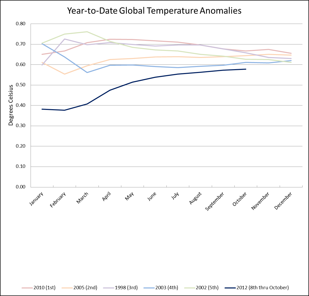


 September 2012 Selected Climate


 and its changes from 2000 to 2050 (20-year average) under the SRES A2 scenario.")
 to 2050 (averages of 2041-2060).")
 and habitat temperature predicted from the growth model presented in this study (filled dots, solid line) and observations (open dots, broken line).")
 ) of marine fishes and invertebrates is fundamentally limited by the balance between energy demand and supply, where
  is reached when energy demand?=?energy supply (thus net growth?=?0). This can be expressed by the function that is commonly used to describe growth of fishes

 are weight at age t and asymptotic weight, respectively; K is the growth parameter that represents the rate of approaching
  through growth.
 and K of marine fishes under scenarios of future water temperature and oxygen level (see
 is smallest in the tropics and approximately five and two times larger in the northern and southern temperate regions, respectively (
 is projected to decrease by 14–24% from 2001 to 2050 (20-year average) or 2.8–4.8%?decade?1 (
 in the tropics are predicted to be large, with an average reduction of around 20% from 2001 to 2050 (20-year average;
  , there is a generally high level of agreement (coefficient of variation <20%) in the projections generated from using the two different earth system models (
 within each fish population, our study shows that most (>75%) of the studied populations are expected to experience a reduction of their
  of 5–39%, with a median of 10% in all ocean basins (
 is larger for fishes in the Pacific and Southern oceans, followed by those in the Atlantic, Indian and Arctic oceans (
 and species composition—contributes around half of the projected body weight shrinkage at the assemblage-level. Out of the 20% average assemblage-level shrinkages by 2050, around 10% is explained by the individual-level shrinkages from increased oxygen demand and reduced oxygen supply, because of the projected warming and reduced oxygen content (
 ) and habitat temperature predicted from the growth model presented in this study (filled dots, solid line) and observations (open dots, broken line).
 induced by climate and ocean changes on marine ecosystems. Assumptions and simplifications of the complex biological system underlying this study are inevitable if we are to make steps toward a better understanding of the effects of global change on marine biota. Such a study, however, provides the foundation for future work, incorporating other mechanisms and factors, and ultimately improving our ability to assess the effects of climate change on biological systems.
 exacerbates the impacts of distribution and abundance change on marine ecosystems. Previous studies identified that the tropics will suffer most from a high rate of local extinction and reduction in maximum catch potential, whereas higher latitude regions, such as the northern temperate regions, may gain
 and log(K) should be negatively and linearly related, and log(K) is negatively related to the inverse of temperature (1/T; see
  and K (
 is clearly demonstrated from empirical analysis of fish’s growth parameters. Such analysis show significant intra-specific relationships between
  and log(K) (see ref.
  and K under changing temperature.
 and von Bertalanffy growth parameter K (see
  , sea water temperature and oxygen content of the habitat and their changes over time, we applied equation (3) to predict changes in
  as a result of changes in ocean conditions for fish populations. Moreover, changes in fish distributions were modelled by the Dynamic Bioclimate Envelope Model (see
  and K; see ref.
 is the maximum body weight of species j. The projected future level of biomass was calculated by multiplying C by the predicted relative abundance (Abd) from the DBEM under climate and ocean changes. The values of W?i are calculated for each year from 1971 to 2060.

Climate Change And Global Warming
Greenpeace says:
Stop Global Warming
We are changing our planet in a fundamental way. Our world is hotter today than it has been in two thousand years.
By the end of the century, if current trends continue, the global temperature could climb so high that the climate and weather patterns that have given rise to human civilization would be radically different.
But it didn’t happen on its own. We’re driving climate change by burning fossil fuels like coal and oil. In fact, coal-fired power plants are the single largest U.S. source of global warming pollution.
America’s coal-burning power plants, in addition to causing global warming and climate change, are killing tens of thousands of Americans, poisoning our air and water, and making our children sick.
But a brighter future is possible. Over the next three years, Greenpeace will:
1. Join local communities to shut down dangerous, dirty coal plants all across the United States.
2. Advocate for strong laws to curb global warming and put America on a path to clean energy.
3. Expose climate deniers, like the Koch Brothers, and hold them publicly accountable for providing millions of dollars to lobby against climate and clean energy policies.
4. Kick-start an Energy Revolution by advocating for clean-energy solutions like solar and wind power.